Problem
4.
(a)
Generate the data for LMS algorithm using the model
To
generate the data drive the above system by a Gaussian white process
with zero mean and a preselected variance. Determine how long you
need to run the system, so that it has reached steady state. Once in
steady, start collecting the data. Collect, at least, 512 points.
(b)
Get an estimate for the signal energy for the above data, and
using this estimate determine range for
 .
Select two values for
.
Select two values for
 in
this range.
in
this range.
(c)
Run the LMS algorithm in the predictive mode for the data that
you have generated and for the two choices of the adaptation gain
.
(d)
Do a validation test. You should use the following for the purpose
of comparison,
Learning
curve (i.e. mean square error curve).
Convergent
values of.
Whiteness
of the error.
Comment
on which choice of gives
better results, and why.
gives
better results, and why.
Solution
(a)
Generation of coloured noise and check for stationarity:
To
generate the coloured noise sequence a Gaussian white noise sequence
and a uniformly distributewhite noise sequence are passed through the
filter given by the transfer function .
Stationarity can be checked by looking at the ensemble mean
sequence and the ensemble correlation function of the
generated data. To get the ensemble mean and auto-correlation the
data is generated 500 times and the average value of the
generated noise
.
Stationarity can be checked by looking at the ensemble mean
sequence and the ensemble correlation function of the
generated data. To get the ensemble mean and auto-correlation the
data is generated 500 times and the average value of the
generated noise for
each value of
for
each value of is
taken as the ensemble mean, while the average value of
is
taken as the ensemble mean, while the average value of for
each
for
each is
taken as the ensemble auto-correlation. The noisy data is generated
for 200 samples, i.e.,
is
taken as the ensemble auto-correlation. The noisy data is generated
for 200 samples, i.e., .
Following are the results obtained MATLAB simulation.
.
Following are the results obtained MATLAB simulation.
Simulation
data:
Generated
data length, L=200
Number
of independent experiments, N=500
Results:
For
Gaussian white noise input:
The
input noise is generated using the MATLAB inbuilt random number
generator,
u=randn(L,1);
Since,
the 'state' of the pseudo-random number generator keeps changing each
time it is called, unless it is specified, the white noise input is
guaranteed to be different each time.
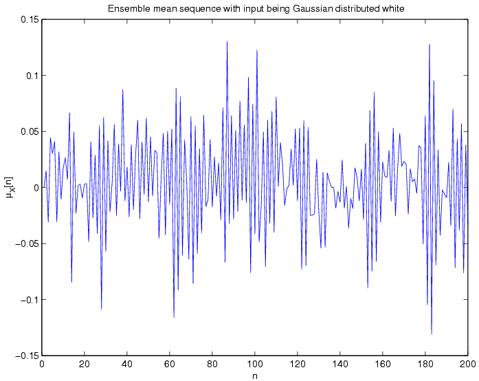
Ensemble
mean sequence:
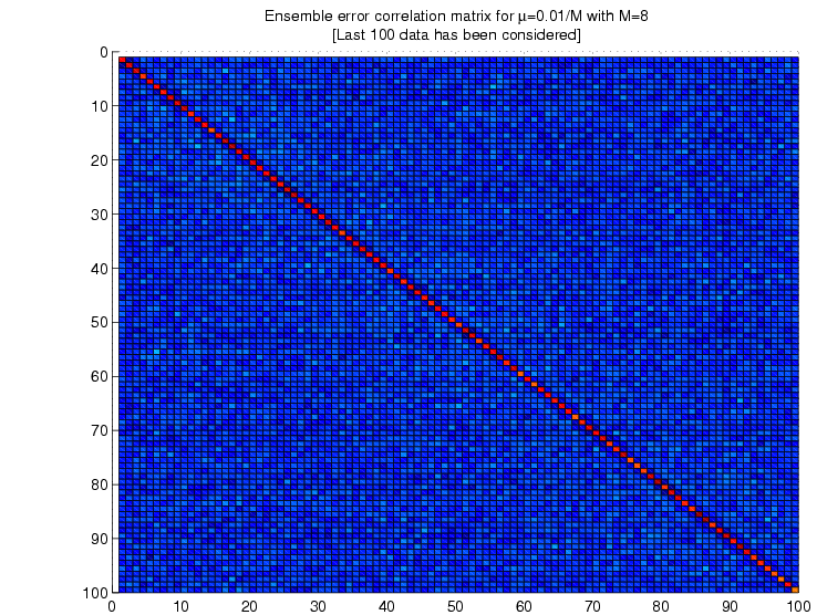
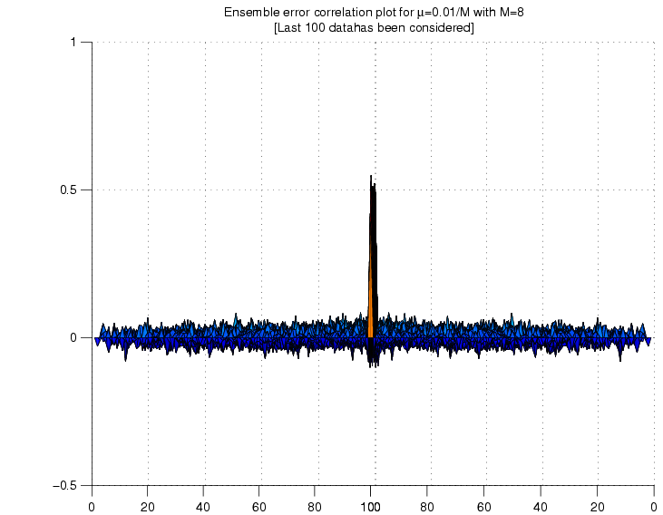
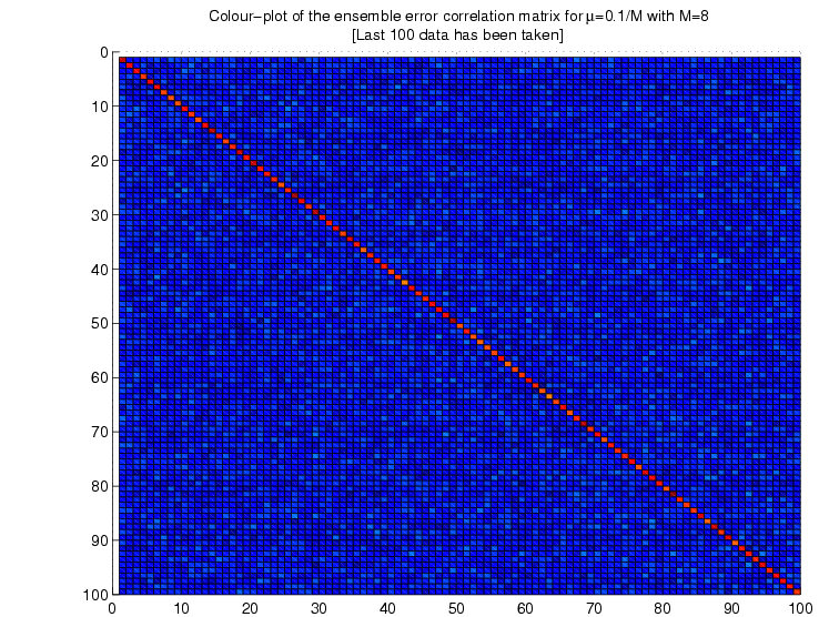
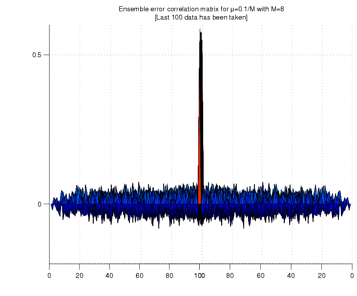
Ensemble
correlation matrix:
The
figures below show the ensemble correlation matrix as an image where
the colour is determined by the value at each cell, for example black
corresponds to zero.
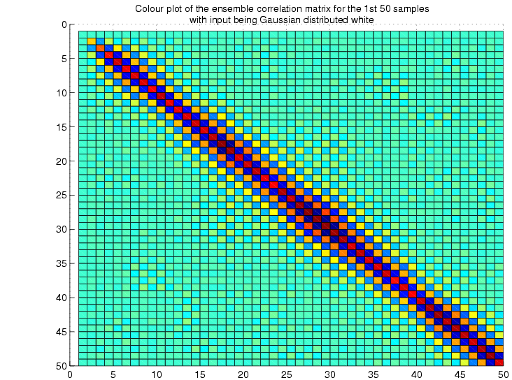
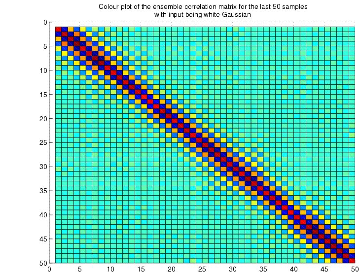
The
toeplitz structure of the matrix is quite evident from the
above two figures.
For
uniformly distributed white noise input:
Here
the white noise is generated by the following command,
u=rand(L,1);
The
stationarity aspect becomes more evident in this case.
Ensemble
mean sequence:
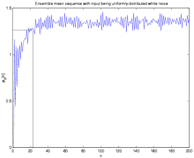
The
mathematical expression for the mean sequence is given by, ,
that is the convolution of the filter impulse response and the input
noise mean sequence. The above figure shows that
,
that is the convolution of the filter impulse response and the input
noise mean sequence. The above figure shows that indeed
settles down after 25 samples, which is in agreement with the
mathematical expression also because in this case
indeed
settles down after 25 samples, which is in agreement with the
mathematical expression also because in this case is
a step function of amplitude 0.5.
is
a step function of amplitude 0.5.
Ensemble
correlation matrix:
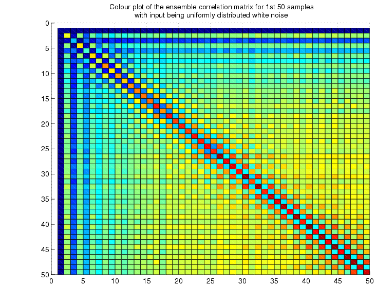
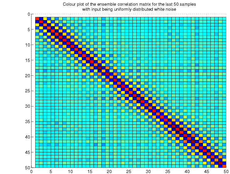
The
above two figures show how the ensemble correlation matrix becomes
toeplitz after almost 25 samples. This toeplitzness, in fact,
is a measure of the stationarity.
(b)
Estimate of the signal power and choice of the adaptation gain, :
:
While
generating the coloured noise, we normalize it so that it has unity
variance in time. This is done so that we can use the samefor
all the realizations. A conservative bound foris
given by, ,
where
,
where is
the filter order and
is
the filter order and is
the estimated signal power. For our simulation we have used two
values of the adaptation gain,as
is
the estimated signal power. For our simulation we have used two
values of the adaptation gain,as and
and .
.
(c)
Running the LMS adaptive predictor:
We
have run the LMS filter as a one step predictor for the coloured
noise generated by passing a Gaussian white noise through the filter
given in the problem.
We
have used the following in the simulation,
Generated
coloured noise length,
Number
of independent experiments,
Number
of initial samples left for the data to become stationary,
Filter
size,

(d)
Validation check:
1.
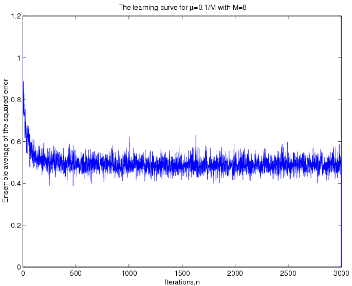
Learning curve: After running the adaptive filter we calculate
the ensemble average of the squared error for each value
of after
after .
This ensemble mean of the squared error is known as the learning
curve of the filter. The figure below shows the learning curve
for the two
s
that we had chosen.
.
This ensemble mean of the squared error is known as the learning
curve of the filter. The figure below shows the learning curve
for the two
s
that we had chosen.
Case
I :
:
Case
II :
:
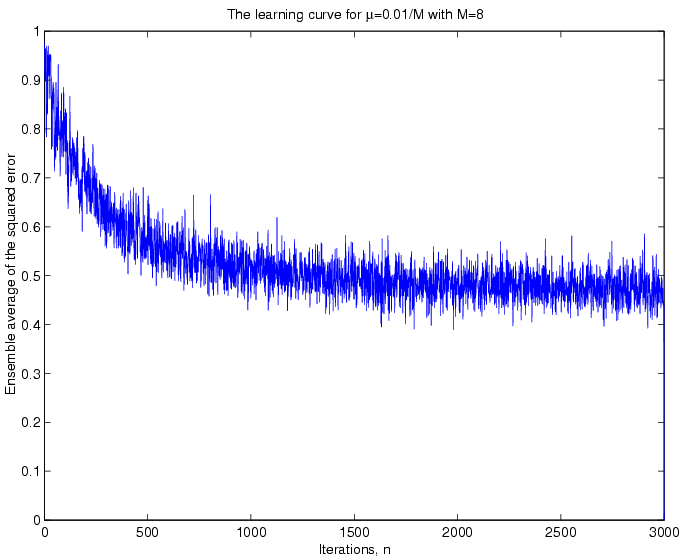
Comparison:
Some of the striking features of the LMS filter revealed by the
two learning curves shown above are enumerated below,
The
squared error oscillates around to 0.5 for ,
whereas it oscillates around 0.49 for
,
whereas it oscillates around 0.49 for ,
i.e., a greatercauses
a greater mean squared error for a given filter order. This fact,
indeed, agrees with the theoretical analysis, which says the
misadjustment
,
i.e., a greatercauses
a greater mean squared error for a given filter order. This fact,
indeed, agrees with the theoretical analysis, which says the
misadjustment
The
convergence is faster for a higher value
 .
.
The
mse approaches the Wiener optimal mse, ,
which can be obtained from the ensemble correlation matrix of the
generated coloured noise for an 8 tap filter. In our case it turns
out that,
,
which can be obtained from the ensemble correlation matrix of the
generated coloured noise for an 8 tap filter. In our case it turns
out that,
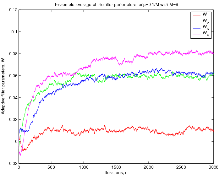
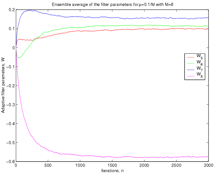
2.
Convergent values of W: The figures below show the convergence of
the ensemble average of the filter parameters.
Case
I:
Case
II
:
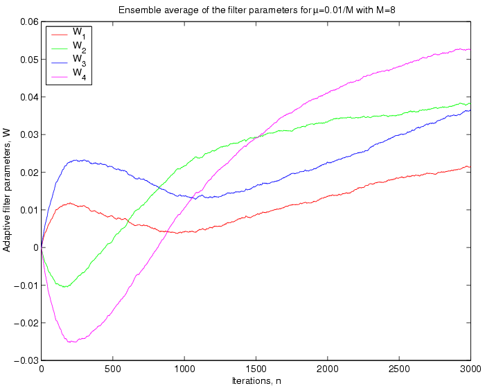
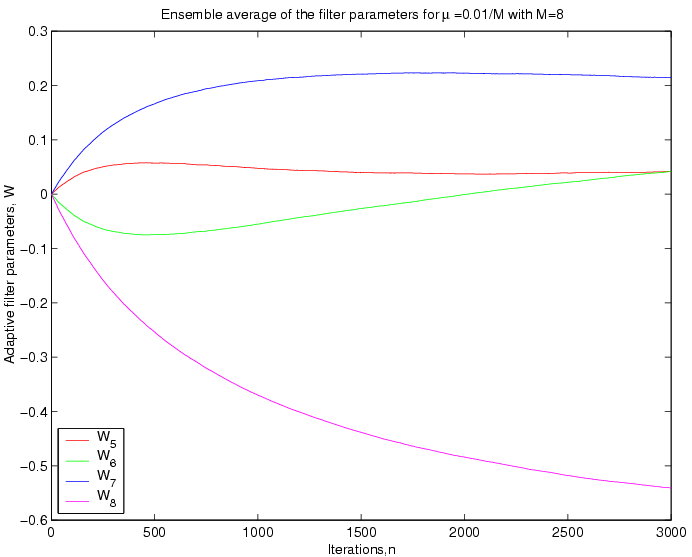
Discussions:
From the above plots it can be seen that for a greater value
ofthe
filter parameters oscillates more. This fact is reasonable, beacuse
thedetermines
the step size of the update in the filter dynamic model, so for a
greaterat
each iteration the change in the
 s will be greater.
The
filter parameters, indeed, approach the Wiener optimal solution,
which can be obtained from ensemble correlation of the generated
coloured noise by solving the Wiener-Hopf equation as given below,
2.
Whiteness of the error: We calculate the ensemble autocorrelation
of the error for last 1000 samples.
Case
I :
:
Case
II