Simulation for Home work 7 Q5

				         Simulation for Home work 7 Problem 5a




Q5 (a) The channel is no longer as given by the cosine function. But, now let the channel be modeled by an FIR filter of 
length 10, and each FIR coefficient be of unit magnitude. This way we will be considering the perfomance of 
the equalizer under a narrow band channel.

Solution

Table for various combinations of F, LMS Order and Variance.
S.No	F	LMS Order	Variance	BER	MSE Plot	Weight Plot	Weights
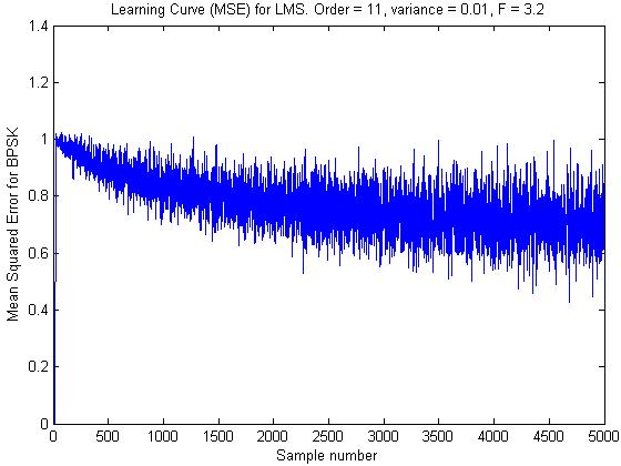
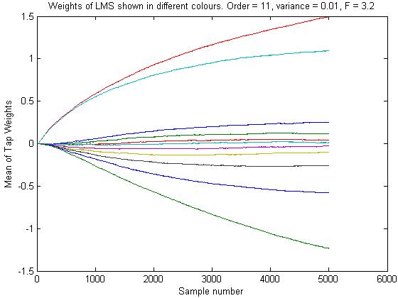
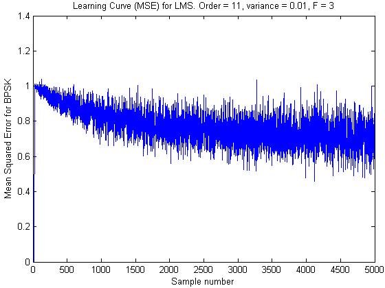
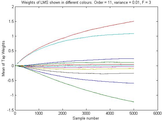
1	3.2	11	0.01	0.2828	mse	weight	0.2489 0.1156 0.0424 0.0124 -0.0255 -0.0987 -0.2585 -0.5784 -1.2335 1.4961 1.0925
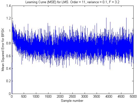
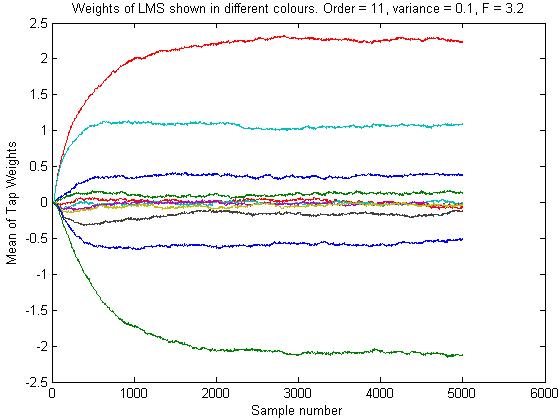
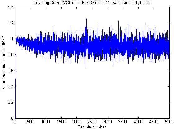
2	3.2	11	0.1	0.2814	mse	weight	0.3802 0.1314 -0.0703 -0.0052 -0.0286 -0.0454 -0.1180 -0.5105 -2.1234 2.2387 1.0892
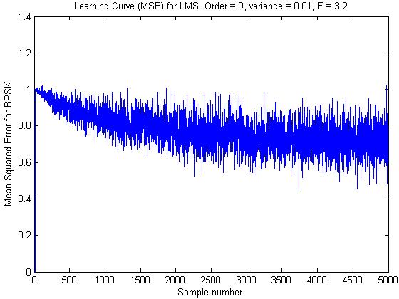
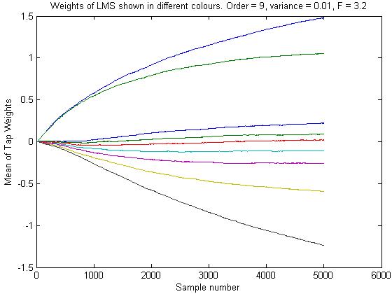
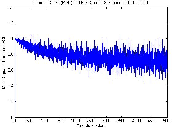
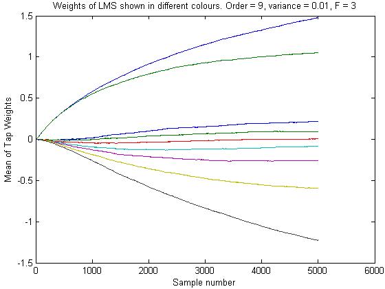
3	3.2	9	0.01	0.2839	mse	weight	0.2213 0.0886 0.0207 -0.1067 -0.2592 -0.5943 -1.2378 1.4793 1.0505
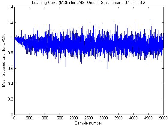
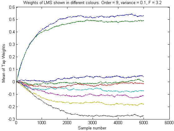
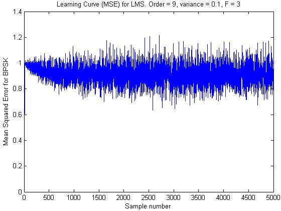
4	3.2	9	0.1	0.3771	mse	weight	0.0406 0.0016 -0.0149 -0.0709 -0.1095 -0.1768 -0.2701 0.5317 0.4916
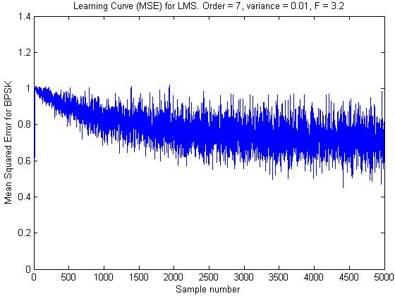
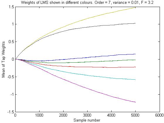
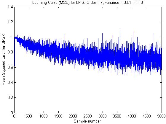
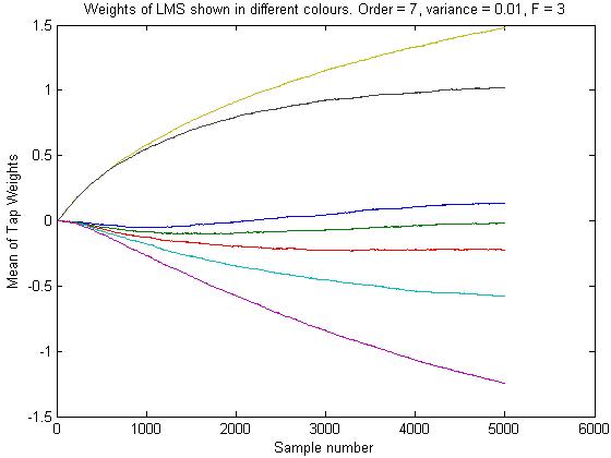
5	3.2	7	0.01	0.2840	mse	weight	0.1502 -0.0185 -0.2217 -0.5815 -1.2246 1.4798 1.0248
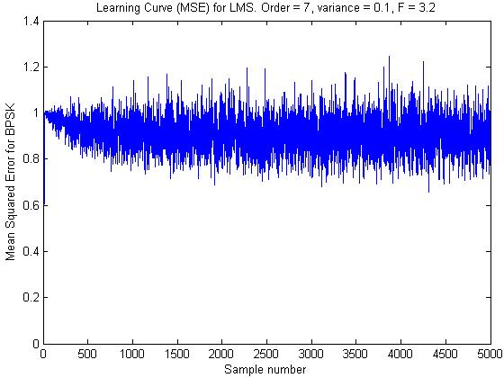
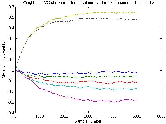
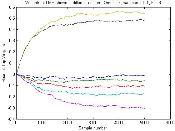
6	3.2	7	0.1	0.3736	mse	weight	-0.0211 -0.0551 -0.1145 -0.1754 -0.2795 0.5520 0.4761
7	3	11	0.01	0.2817	mse	weight	0.2447 0.1153 0.0449 0.0189 -0.0290 -0.0960 -0.2545 -0.5925 -1.2253 1.5042 1.0882
8	3	11	0.1	0.3775	mse	weight	0.0619 0.0529 0.0223 -0.0141 -0.0392 -0.0521 -0.1123 -0.1836 -0.2929 0.5544 0.4876
9	3	9	0.01	0.2860	mse	weight	0.2180 0.0914 0.0085 -0.0823 -0.2573 -0.5939 -1.2251 1.4806 1.0537
10	3	9	0.1	0.3761	mse	weight	0.0210 0.0067 -0.0350 -0.0758 -0.0922 -0.1893 -0.2761 0.5299 0.4888
11	3	7	0.01	0.2856	mse	weight	0.1354 -0.0168 -0.2221 -0.5786 -1.2452 1.4783 1.0207
12	3	7	0.1	0.3742	mse	weight	-0.0094 -0.0552 -0.1021 -0.1749 -0.3013 0.5441 0.4864

Q5 (a) The channel is no longer as given by the cosine function. But, now let the channel be modeled by an FIR filter of length 10, and each FIR coefficient be of unit magnitude. This way we will be considering the perfomance of the equalizer under a narrow band channel.