Code for performing simulations
Krishna Subramani, Yashswi Jain
- The following notebook contains the code to perform the solutions and obtain the plots and results.
- There are detailed description cells and comments detailing what section of the code does what.
- The data needs to be in the same directory as this notebook
import matplotlib.pyplot as pyp
import numpy as np
import time
# Extracting data parameters from the csv files
import csv
import glob
# Function to calculate distances given the latitude and longitude
from math import cos, asin, sqrt
def distance(lat1, lon1, lat2, lon2):
    p = 0.017453292519943295     #Pi/180
    a = 0.5 - cos((lat2 - lat1) * p)/2 + cos(lat1 * p) * cos(lat2 * p) * (1 - cos((lon2 - lon1) * p)) / 2
    return 12742 * asin(sqrt(a)) #2*R*asin...
Data Scavenging
One of the major challenges in the project was availability of free sanitised data. Almost all the environmental websites didn't have free data available for download. The best possible data that was found had stations which were encoded in a particular format which had to be decoded to get the latitude and longitude values.
Procedure followed in extracting the data -
- The csv files are parsed to extract the latitude and longitude information of the weather centres.
- Then, the sensor data is extracted from the csv files. If the data value is 'NULL', that value is imputed with the previous valid sensor value replacing the current value.
- Here the parameters are $N_1 = 30$ and $N_2 = 400$ where $N_1$ is the number of sensors and $N_2$ is the number of time instants for which the sensor values are considered(here, 400 means 400 days)
list_csv_files = glob.glob("./Data/*.csv")
altitude = []
coordinates = []
data = [] # Time series

num_files = len(list_csv_files)

# Frame size in moving average in data imputation
W = 5

num_data = 400
for item in list_csv_files:
    fields = []
    rows = []
    with open(item, 'r') as csvfile:
        # creating a csv reader object
        csvreader = csv.reader(csvfile)
        for row in csvreader:
            rows.append(row)
    altitude.append((int)(rows[0][1][0:3]))
    coordinates.append([(int)(rows[1][1][0:2]) + (int)(rows[1][1][3:5])*1.0/60,(int)(rows[2][1][0:2]) + (int)(rows[2][1][3:5])*1.0/60])
    cou = 0
    temp = []
    for i in rows[6:]:
        if(cou == num_data):
            break
        if(i[1] != 'NULL'):
            temp.append((float)(i[1]))
#             cou = cou + 1
        else:
#             continue
            if(cou==0):
                temp.append(0)
            else:
                temp.append(temp[cou-1])
        cou = cou + 1
    data.append(temp)
altitude[0] = 1159
# Sample plot of the sensors reading at one of the stations for N = 200 days.
pyp.plot(data[28])
pyp.title('Example of Sensor Readings across 400 days')
pyp.ylabel('Sensor Temperature(C)')
pyp.xlabel('Number of Days');
# pyp.savefig('Images\SensorData_example.png')

Laplacian Construction -
We have tried 5 different ways of caclulating the weight matrix from the distance matrix of the weather stations -
- We use the Weight matrix as it is for the Distance Matrix D
- We use the normalized weight matrix i.e. the Distance matrix D is divided by the max value $D = D/D_{maxval}$
- We calculate the weight matrix based on the following formula $W_{i,j} = Ke^{-|d_{i} - d_{j}|/D_{max}}$
- Weight matrix calculated based on the altitudes as opposed to the ground distances.
- Nearest Neighbour weight matrix : for each node, only keep the N nearest neighbours.
# Choosing which of the above method is wanted to construct the Laplacian(2 by default)
choice = 5
# Forming the Distance Matrix
D = np.zeros((num_files,num_files))
W3 = np.zeros((num_files,num_files))
K = 1
for i in range(num_files):
    for j in range(num_files):
        D[i,j] = distance(coordinates[i][0],coordinates[i][1],coordinates[j][0],coordinates[j][1])

# d_sort = np.sort(D(0))
D1 = D
#simple distance metric

maxval = np.max(D)

D2 = D/maxval
#normalised d value
for i in range(num_files):
    for j in range(num_files):
        W3[i,j] = K*np.exp(-1*distance(coordinates[i][0],coordinates[i][1],coordinates[j][0],coordinates[j][1])/maxval)
W3 = W3 - np.eye(num_files,num_files)
#weight is exp()

D4 = np.zeros((num_files,num_files))
for i in range(num_files):
    for j in range(num_files):
        D4[i,j] = (altitude[i] - altitude[j])**2
D4 = D4 - np.eye(num_files)
maxval = np.max(D4)
D4 = D4/maxval
#d4 is the alt difference matrix

# Nearest Neighbour graph using the exopnentially weighted matrix above
#Wd = W3
wd = D4
# Number of neighbours to keep
nneb = 10
for i in range(num_files):
    for j in range(i+1,num_files):
        vals = np.sort(W3[i,:])
        if(Wd[i,j] < vals[-nneb]):
            Wd[i,j] = 0
            Wd[j,i] = 0

# Constructing the Laplacian matrix L from the above calculated weight matrices
L1 = np.diag((np.sum(D1,0))) - D1 #simple distance metric
L2 = np.diag((np.sum(D2,0))) - D2#normalised distance
L3 = np.diag((np.sum(W3,0))) - W3#exp weights
L4 = np.diag((np.sum(D4,0))) - D4#alt diff.
L5 = np.diag((np.sum(Wd,0))) - Wd#nearest neighbor using alt diff.

if(choice == 1):
    L = L1
elif(choice == 2):
    L = L2
elif(choice == 3):
    L = L3
elif(choice == 4):
    L = L4
else:
    L = L5
### Displaying the obtained Laplacian(to see if there is any visible structure in the distances)
pyp.imshow(L)
pyp.colorbar()
pyp.title('Heat map of Graph Laplacian for Sensor Network')
pyp.ylabel('Sensor i')
pyp.xlabel('Sensor j');
pyp.savefig('Images\graph_laplacian_dist_metric.png')

Constructing the Time-Series graph -
From the reference paper, the time series graph is essentially a node for each time sample and it is a directed graph. The following figure is from the paper -
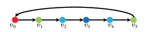
The final loopback is to indicate that the data is periodic. In our case however, the data need not be periodic. Hence, we do not perform the last loopback.
Another thing not mentioned in the reference paper is what the weights of the digraph should be taken as. Hence, as a starting point, we assume the weights to be one in this case.
Wt = np.zeros((num_data,num_data))
for i in range(num_data):
    for j in range(num_data):
        if((j - i) == 1):
            Wt[i,j] = 1
Lt = np.diag((np.sum(Wt,0))) - Wt
Lt[0,0] = 1
pyp.imshow(Lt[0:10,0:10])
pyp.colorbar()

Graph Product Factorization -
We now invoke the primary assumption from the paper i.e. the overall graph consisting of the $N_1 = 30$ sensor values across the $N_2 = 400$ time instants can be written as the 'Strong Product' of the two following graphs - 1) The sensor network graph and 2) The time series graph. We state below the following equation from the paper ($\otimes$ refers to the Matrix Kronecker product) -
\begin{align}
&L_{\oplus} = L_{1} \otimes L_{2} + L_{1} \otimes I_{N_2} + L_{2} \otimes I_{N_1}\\
\end{align}
After diagonalizing the individual graph Laplacians to obtain the individual representations, the overall representation can be written in the following way -
\begin{align}
&L_{\oplus} = V \times \left( \Lambda_{1} \otimes \Lambda_{2} + \Lambda_{1} \otimes I_{N_2} + I_{N_1} \otimes \Lambda_{2} \right) \times V^{-1}\\
\end{align}
Where $\Lambda_{1},\Lambda_{2}$ are the individual graph laplacian eigenvalue matrices, and $V = V_{1} \otimes V_{2}$ is the Kronecker product of the individual graph Laplacian eigenvector matrices
Similar to the above, we can also relate the Fourier Transform of the graph products to the individual transforms in the following way -
\begin{align}
&V^{-1} = \left( V_{1} \otimes V_{2} \right) ^{-1} = V_{1}^{-1} \otimes V_{2}^{-1}
\end{align}
[u1,s1,v1] = np.linalg.svd(L)
[u2,s2,v2] = np.linalg.svd(Lt)
l1 = np.diag(np.sqrt(s1))
l2 = np.diag(np.sqrt(s2))
Vp = np.kron(u1,u2)
Lp = np.kron(l1,np.eye(l2.shape[0])) + np.kron(np.eye(l1.shape[0]),l2) + np.kron(l1,l2)
V_trans = Vp
After obtaining the effective eigenvalue matrix $\Lambda = \Lambda_{1} \otimes \Lambda_{2} + \Lambda_{1} \otimes I_{N_2} + \Lambda_{2} \otimes I_{N_1}$, we observe that the eigenvalues are not in a sorted order. Hence, to interpret them as some sort of 'frequency' measure, we sort the eigenvalues in the ascending order and at the same time, we rearrange the following eigenvectors as well.
Compression in the Frequency domain
Once we have obtained the above matrices, which essentially correspond to the transformation matrix and eigenvalue matrix for the overall graph, we follow the following steps to perform the compression.
- We first define the $N_{1} \times N_{2}$ graph signal as the time series signal at all the $N_1$ stations for all the $N_2$ time instants. We unroll this into a single vector to obtain the 'effective' graph signal for the overall graph.
- Then, we take this unrolled vector into the spectral domain using the above obtained transformation. We then only keep the k components with the highest coefficient magnitudes and then reconstruct the signal using the inverse transformation.
- Then, we compute the following for varying values of k - \begin{align} &e_{p} = \frac{|x_{or} - x_{recon}|}{|x_{or}|}\\ \end{align} Here the above quantity is the Compression error(lower is better)
# GFT by inverse of the smaller matrices
# Define the number of components to consider in the frequency spectrum
time_start = time.time()
lst = [1,0.9,0.85,0.8,0.75,0.7,0.6,0.5,0.4,0.3,0.2,0.15,0.1,0.07,0.05,0.002]
lst = np.asarray(lst)
lst = (np.floor(lst*num_files*num_data)).astype(int)
mseall = []
msepall = []
psnr = []
for k in lst:
    #print(k)
    bb = np.matrix(data)#Original
    bcb = np.reshape(bb,(num_files*num_data,1))
    bcb = bcb - np.mean(bcb)#Zero meaning
    Vfur = np.kron(np.linalg.inv(u1),np.linalg.inv(u2))
    recon_data = np.matmul(Vfur,bcb)#Fourier Transforming
    lvals = np.sort(np.abs(np.asarray(recon_data).ravel()))#Finding the dominant Fourier coefficients
    thresh = lvals[-k]
    low_values_flags = abs(recon_data) < thresh
    recon_data[low_values_flags] = 0;
    recon_data = np.matmul(Vp,recon_data);
    mse = np.linalg.norm(bcb - recon_data)
    msep = mse/np.linalg.norm(bcb)
    mseall.append(mse)
    msepall.append(msep*100)
    psnr.append(10*np.log10(np.max(np.abs(bcb)*2)/mse))
time_end = time.time()
print("Time taken to inverse the small matrix is : ",(time_end - time_start)/(60.0*len(lst)))
pyp.figure()
pyp.plot(lst/(num_files*num_data),msepall)
# pyp.title('Reconstruction Error without clipping')
pyp.xlabel('Fraction of Components considered')
pyp.ylabel('Error Percentage')
pyp.grid()
pyp.ylim([0,100])
pyp.savefig('Images\error_withoutclipping_KNN_altDiff..png')

In the above plot, Notice the Error is 0 if 100% of the data is used for reconstruction which conforms to the expectation. For 80% of the data, the Reconstruction error is less 5%, hence accuracy of >95% for a compression of about 20%, further, the accuracy is ~ 75% for as less as ~25% of data i.e. a compression of about 75%.
# GFT by inverse of the bigger matrix
time_start = time.time()
# Define the number of components to consider in the frequency spectrum
lst = [1,0.9,0.85,0.8,0.75,0.7,0.6,0.5,0.4,0.3,0.2,0.15,0.1,0.07,0.05,0.002]
lst = np.asarray(lst)
lst = (np.floor(lst*num_files*num_data)).astype(int)
mseall = []
msepall = []
psnr = []
for k in lst:
    #print(k)
    bb = np.matrix(data)#Original
    bcb = np.reshape(bb,(num_files*num_data,1))
    bcb = bcb - np.mean(bcb)#Zero meaning
    recon_data = np.matmul(np.linalg.inv(V_trans),bcb)#Fourier Transforming
    lvals = np.sort(np.abs(np.asarray(recon_data).ravel()))#Finding the dominant Fourier coefficients
    thresh = lvals[-k]
    low_values_flags = abs(recon_data) < thresh
    recon_data[low_values_flags] = 0;
    recon_data = np.matmul(Vp,recon_data);
    mse = np.linalg.norm(bcb - recon_data)
    msep = mse/np.linalg.norm(bcb)
    mseall.append(mse)
    msepall.append(msep*100)
    psnr.append(10*np.log10(np.max(np.abs(bcb)*2)/mse))
time_end = time.time()
print("Time taken to inverse the bigger matrix is : ",(time_end - time_start)/(60*len(lst)))
Outlier Removal using Interquartile Range Clipping
We will first display the boxplot of the sensor values for a single station. Based on the obtained plot, we can clip the values outside the majority ranges to a fixed value to reduce the impact of outliers on the compression.
pyp.subplot(2,1,1)
pyp.boxplot(data[1])
pyp.subplot(2,1,2)
pyp.boxplot(data[2]);

The orange line represents the mean, and the box around it represents the interquartile range(0.25 percentile to 0.75 percentile). The black lines above are 1.5 times the interquartile range.
The data corresponding to the first sensor shows no outliers, however the data corresponding to the second sensor has a few outliers.
data_m = np.asmatrix(data)
data_m = data_m.T
for i,v in enumerate(data):
    q1, q3= np.percentile(v,[25,75])
    iqr = q3 - q1;
    thresh = 1.5
    lower_bound = q1 - (thresh * iqr)
    upper_bound = q3 + (thresh * iqr) # 1.5 times can be changed
    data_m[:,i][data_m[:,i] <= lower_bound] = lower_bound
    data_m[:,i][data_m[:,i] >= upper_bound] = upper_bound
# Define the number of components to consider in the frequency spectrum
time_start = time.time()
lst = [1,0.9,0.85,0.8,0.75,0.7,0.6,0.5,0.4,0.3,0.2,0.15,0.1,0.07,0.05,0.002]
lst = np.asarray(lst)
lst = (np.floor(lst*num_files*num_data)).astype(int)
mseall = []
msepall = []
psnr = []
for k in lst:
    #print(k)
    bb = np.matrix(data_m)#Original
    bcb = np.reshape(bb,(num_files*num_data,1))
    bcb = bcb - np.mean(bcb)#Zero meaning
    Vfur = np.kron(np.linalg.inv(u1),np.linalg.inv(u2))
    recon_data = np.matmul(Vfur,bcb)#Fourier Transforming
    lvals = np.sort(np.abs(np.asarray(recon_data).ravel()))#Finding the dominant Fourier coefficients
    thresh = lvals[-k]
    low_values_flags = abs(recon_data) < thresh
    recon_data[low_values_flags] = 0;
    recon_data = np.matmul(Vp,recon_data);
    mse = np.linalg.norm(bcb - recon_data)
    msep = mse/np.linalg.norm(bcb)
    mseall.append(mse)
    msepall.append(msep*100)
    psnr.append(10*np.log10(np.max(np.abs(bcb)*2)/mse))
time_end = time.time()
print("Time taken to inverse the small matrix is : ",(time_end - time_start)/(60.0*len(lst)))
pyp.figure()
pyp.plot(lst/(num_files*num_data),msepall)
# pyp.title('Reconstruction Error with clipping')
pyp.xlabel('Fraction of Components considered')
pyp.ylabel('Error Percentage')
pyp.grid()
pyp.ylim([0,100])
pyp.savefig('Images\error_clipping.png')

ind = 28
q1, q3= np.percentile(data[ind],[25,75])
iqr = q3 - q1;
thresh = 1.5
lower_bound = q1 - (thresh * iqr)
upper_bound = q3 + (thresh * iqr) # 1.5 times can be changed
pyp.subplot(2,1,1)
pyp.boxplot(data[ind])
pyp.subplot(2,1,2)
pyp.plot(data[ind])
pyp.axhline(lower_bound,color = 'r')
pyp.axhline(upper_bound,color = 'r')
# pyp.title('Sensor data and boxplot')
pyp.xlabel('Day number')
pyp.ylabel('Sensor Temperature')
pyp.savefig('Images\data_bp.png')
