Current method used in Literature :
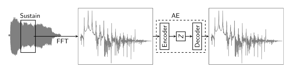
The above framewise magnitude spectra reconstruction procedure is described in [1]. We implemented it as shown, and observe that the reconstruction cannot generalize to pitches the network has not been trained on. For demonstration, we train the network including and excluding MIDI 63 along with its 3 neighbouring pitches on either side :
(a) Including MIDI 63
| MIDI | 60 | 61 | 62 | 63 | 64 | 65 | 66 |
|---|---|---|---|---|---|---|---|
| Kept | $\checkmark$ | $\checkmark$ | $\checkmark$ | $\checkmark$ | $\checkmark$ | $\checkmark$ | $\checkmark$ |
(b) Excluding MIDI 63
| MIDI | 60 | 61 | 62 | 63 | 64 | 65 | 66 |
|---|---|---|---|---|---|---|---|
| Kept | $\checkmark$ | $\checkmark$ | $\checkmark$ | $\times$ | $\checkmark$ | $\checkmark$ | $\checkmark$ |
We then give MIDI 63 as an input to both the above cases, and see how well the network can reconstruct the input
import IPython.display as ipd
print('Input MIDI 63 Note')
ipd.display(ipd.Audio('./ex/D#_19_og.wav'))
print('(a) Reconstructed MIDI 63 Note when trained Including MIDI 63')
ipd.display(ipd.Audio('./ex/D#_19_trained_recon_stft_AE.wav'))
print('(b) Reconstructed MIDI 63 Note when trained Excluding MIDI 63')
ipd.display(ipd.Audio('./ex/D#_19_skipped_recon_stft_AE.wav'))
%%HTML
<a href="./ex/Ds_19_og.png" target="_blank">Input MIDI 63 Spectrogram</a> <br>
<a href="./ex/Ds_19_trained_recon.png" target="_blank">(a) Reconstructed MIDI 63 Spectrogram when trained Including MIDI 63</a> <br>
<a href="./ex/Ds_19_skipped_recon.png" target="_blank">(b) Reconstructed MIDI 63 Spectrogram when trained Excluding MIDI 63</a> <br>
On hearing the reconstructed version of the input note, and glancing at the spectrogram, you can clearly see that the frame-wise magnitude spectrum based reconstruction procedure cannot reconstruct pitches it has not been trained on. This gives us a good motivation to move on to a parametric model
Proposed Method
Parametric Model
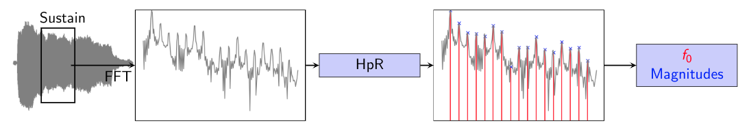
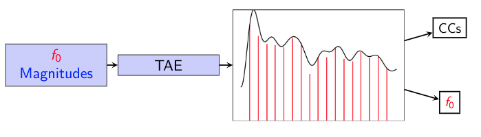 The above shows the Parametric(Source-Filter) representation of a signal. The procedure is described in detail in [2]. The TAE algorithm is described in [3].
The audio clips below show the Parametric reconstruction of an input audio note. As mentioned in the paper, we only work with the harmonic component, and neglect the residual for now
print('Original MIDI 60 Note')
ipd.display(ipd.Audio('./ex/C_3.wav'))
print('Source Filter Reconstructed MIDI 60 Note')
ipd.display(ipd.Audio('./ex/C_3_recon.wav'))
# print('Original F4 Note')
# ipd.display(ipd.Audio('./Audio_SF/F_15.wav'))
# print('Source Filter Reconstructed F4 Note')
# ipd.display(ipd.Audio('./Audio_SF/F_15_recon.wav'))
# print('Original B4 Note')
# ipd.display(ipd.Audio('./Audio_SF/B_15.wav'))
# print('Source Filter Reconstructed B4 Note')
# ipd.display(ipd.Audio('./Audio_SF/B_15_recon.wav'))
Network Architecture
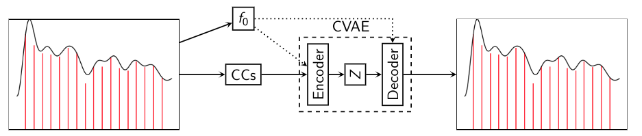
This is our proposed model - VaPar Synth - a Variational Parametric synthesizer which utilizes a Conditional Variational Autoencoder(CVAE) trained on a parametric representation.
We demonstrate the experiments performed ahead.
Experiments
Experiment 1 - Reconstruction
The table below shows training when skipping MIDI 63, and training on its 3 nearest neighbours.
| MIDI | 60 | 61 | 62 | 63 | 64 | 65 | 66 |
|---|---|---|---|---|---|---|---|
| Kept | $\checkmark$ | $\checkmark$ | $\checkmark$ | $\times$ | $\checkmark$ | $\checkmark$ | $\checkmark$ |
We show the input note 63, and the reconstructions by the AE and CVAE. We also show the reconstructions of the spectral envelopes
print('Input MIDI 63 Note')
ipd.display(ipd.Audio('./ex/D#_19_input_pm.wav'))
print('AE reconstruction')
ipd.display(ipd.Audio('./ex/D#_19_recon_AE.wav'))
print('CVAE reconstruction')
ipd.display(ipd.Audio('./ex/D#_19_recon_cVAE.wav'))
%%HTML
<a href="./ex/Ds_19.png" target="_blank">Spectral Envelope(Input and Reconstruction)</a>
On listening to both the audio, you can see that both the AE and CVAE can reconstruct the audio without considerably changing its timbre. If you look at the spectral envelopes as well, both the models are able to capture the overall shape, and follow it closely.
We also train our model only on the endpoints, and skip all the other pitches in the octave, as shown in the table below.
| MIDI | 60 | 61 | 62 | 63 | 64 | 65 | 66 | 67 | 68 | 69 | 70 | 71 |
|---|---|---|---|---|---|---|---|---|---|---|---|---|
| Kept | $\checkmark$ | $\times$ | $\times$ | $\times$ | $\times$ | $\times$ | $\times$ | $\times$ | $\times$ | $\times$ | $\times$ | $\checkmark$ |
Our model reconstructs pitches close to the endpoints similar to the previous one. We show the reconstruction of a pitch which is far away from the train points - MIDI 65, and analyze how the network reconstructs this pitch
print('Input MIDI 65 Note')
ipd.display(ipd.Audio('./ex/F_20_og.wav'))
print('AE reconstruction')
ipd.display(ipd.Audio('./ex/F_20_recon_AE.wav'))
print('CVAE reconstruction')
ipd.display(ipd.Audio('./ex/F_20_recon_cVAE.wav'))
%%HTML
<a href="./ex/F_20.png" target="_blank">Spectral Envelope(Input and Reconstruction)</a>
The AE reconstruction sounds a bit 'spread out'(loosely speaking). The CVAE reconstruction sounds a bit closer to the input. This can also be explained by looking at the spectral envelopes. The CVAE tries to follow the overall shape of the input envelope closer than the AE reconstruction, which peaks around certain frequencies and has more oscillations.
Experiment 2 - Generation
We train the network on the whole octave sans MIDI 65, and we see how well it can generate MIDI 65. We present both the network generate MIDI 65 note, and a similar sounding MIDI 65 from the dataset.
print('Input MIDI 65 Note')
ipd.display(ipd.Audio('./ex/65_ogg.wav'))
print('Network Generated MIDI 65 note')
ipd.display(ipd.Audio('./ex/65_gen.wav'))
The reconstructed note sounds synthetic when compared to the Input note. This is mostly because the generated note is missing soft noisy sound of the bowing. This is expected because we only model the harmonic component and neglect the residual.
We have also added a vibrato to demonstrate that the network can synthesize continuosly varying frequencies.
print('Network Generated MIDI 65 note with vibrato')
ipd.display(ipd.Audio('./ex/65_gen_vibrato.wav'))
Experiment 3 - Timbre Hybridization
The latent space learned by the network allow to continuously represent instrument sounds. If the latent dimensions are related to timbre perception, sampling from different clusters should yield different timbres.
Here is an example of the 2-dimensional latent space we obtained when training on brass and organ sounds from NSynth.

import IPython.display as ipd
print("Brass Sound from the training set")
ipd.display(ipd.Audio("./Work/brassOG.wav"))
print("Brass Sound sampled from the latent space")
ipd.display(ipd.Audio("./Work/brassRecon.wav"))
print("Organ Sound from the training set")
ipd.display(ipd.Audio("./Work/organOG.wav"))
print("Organ Sound sampled from the latent space")
ipd.display(ipd.Audio("./Work/organRecon.wav"))
print("Sweep from brass to organ")
ipd.display(ipd.Audio("./Work/transition1.wav"))
One can hear that the timbre are not clearly different and of subpar quality. However, it is still possible to hear a slight difference between the brass and the organ. Most importantly, we observed that is possible to sample continuously from the latent space, which allows us to hope that our model could technically enable continuous timbre hybridization. Nevertheless, this would require changing the network because a (C)VAE enforces a single Gaussian prior on the latent space that fails to model two different instrument timbres.
References
- Roche, Fanny, et al. "Autoencoders for music sound modeling: a comparison of linear, shallow, deep, recurrent and variational models." arXiv preprint arXiv:1806.04096 (2018).
- Caetano, Marcelo, and Xavier Rodet. "A source-filter model for musical instrument sound transformation." 2012 IEEE International Conference on Acoustics, Speech and Signal Processing (ICASSP). IEEE, 2012.
- Röbel, Axel, and Xavier Rodet. "Efficient spectral envelope estimation and its application to pitch shifting and envelope preservation." 2005.
%%HTML
<script>
function code_toggle() {
if (code_shown){
$('div.input').hide('500');
$('#toggleButton').val('Show Cells')
} else {
$('div.input').show('500');
$('#toggleButton').val('Hide Cells')
}
code_shown = !code_shown
}
$( document ).ready(function(){
code_shown=false;
$('div.input').hide()
});
</script>
<form action="javascript:code_toggle()"><input type="submit" id="toggleButton" value="Show Cells "></form>